Maps of Phase Equilibirum - Binary Isomorphous Phase Diagrams
Sugar and water is a familiar and interesting system, but that phase diagram is probably more relevant to food scientists. Materials scientists and engineers typically work with phase diagrams for metal alloys, ceramic systems, and polymer mixtures. Let's look at perhaps the simplest of phase diagrams - the isomorphous (iso- means "same" and "morphous" means shape or structure) binary phase diagram.
In earlier sections (Section 6.5 and Section 10.3) we found that sometimes, when one atom substitutes for another in a lattice, there is only a small disruption in the host lattice and we can form a complete solid solution. This is a solution that in which one can change the concentration of the impurity from very small to very large values and never yield the formation of a new phase. Copper and nickel are one such pairs that form a complete solid solution: the nickel can substitute into the copper host lattice without leading to a significant disruption structure, and the copper can do the same in the nickel. They are completely miscible. Because they are completely miscible, they have a single phase field in the lower-temperature region from pure nickel to pure copper (Figure 10.6.1). That is, the phase of pure nickel (which has an FCC structure) and the phase of pure copper (which also has an FCC structure) are so structurally similar (i.e. they are isomorphous) that they mix completely.
As is tradition in most introductory MSE courses, we'll use the Cu-Ni phase diagram as a playground to learn about isomorphous phase diagram. Notably, there are really interesting materials in this phase diagram, including cupronickel alloys (used for coinage) and monel (used in marine and chemical processing industries, as well as decorative articles).

Figure 10.6.1 The binary isomorphous phase diagram for the Cu-Ni system. At high temperature, there is a liquid solution phase field $\ell_{\mathrm{s}}$ (light orange), at lower temperature there is a solid solution phase field $\alpha$ (light blue). At the boundary of these two phase fields there is a region in which we have two phases in equilibrium: $\ell_{\mathrm{s}} + \alpha$ (light green).
Phase Fields in Isomorphous Phase Diagrams
Let's look at the phase diagram in Figure 10.6.1 in detail:
-
At lower temperature we observe this region of complete miscibility in Figure 10.6.1. We label it $\alpha$ because in science we like to use Greek letters to represent things; $\alpha$ simply communicates that the material has a specific crystal structure in this phase field. Note - $\alpha$ does not necessarily mean FCC, or BCC, or whatever. Greek letters will represented different crystal structures in different phase diagrams. <\br> If I hold my system at a temperature and composition that places us in the $\alpha$, I expect to only observe a solid solution.
-
At higher temperature, we'd expect the alloy to melt, and so we see, at higher tempreature, a phase field of liquid solution $\ell_{\mathrm{s}}$. Note - the liquid phases of Ag and Cu are also miscible (like water and alcohol), although not all liquid phases need be miscible (like oil and water). <\br> If I hold my system at a temperature and composition that places us in the $\ell_{\mathrm{s}}$, I expect to only observe a liquid solution.
-
At intermediate temperature we have a region of two-phase equilibrium, as denoted by the label $\ell_{\mathrm{s}}+\alpha$. In this region we expect both the liquid phase and the solid phase to be present in equilibrium. <\br> If I hold my system at a temperature and composition that places us in the $\ell_{\mathrm{s}}+ \alpha$, I expect to observe a both a liquid solution and and solid solution.
Phase Boundaries and Melting Points
There's clearly sharp boundaries between these phase fields, denoted by solid lines. We give those phase boundaries names:
- The so-called liquidus separating the $\ell_{\mathrm{s}}$ and $\ell_{\mathrm{s}} + \alpha$ phase fields. Above this line, we only have a liquid phase.
- The so-called solidus separating the $\alpha$ and $\ell_{\mathrm{s}} + \alpha$. Below this line we only have a solid phase.
One can think of these phase boundaries very similarly to the solubility limit in the sugar-water phase diagram on the previous page. We'll discuss this more below.
There are two other points of interest that one should recognize:
- The point at $C = 0 \text{ wt% Ni}$ (pure copper) and $T = 1084 ^{\circ}\text{C}$: the point where we transition from pure, solid copper to pure, liquid copper upon heating. Or, the melting point of copper, labeled $T_{\mathrm{m}}(\text{Cu})$.
- The point at $C = 100 \text{ wt% Ni}$ (pure nickel) and $T = 1452 ^{\circ}\text{C}$: the point where we transition from pure, solid nickel to pure, liquid copper upon heating. Or, the melting point of nickel, labeled $T_{\mathrm{m}}(\text{Ni})$.
The melting points provide an opportunity to navigate these phase diagrams and build some intuation. Let's say we're at $C = 0 \text{ wt% Ni}$ and $T = 1050 ^{\circ}\text{C}$. What phase field are we in? Well, it looks like in the $\alpha$ phase field, or we're solid. Now, we heat our specimen to $T = 1100 ^{\circ}\text{C}$ without changing composition. Now we're in the liquid phase field. Something happened... a phase transition where $\alpha \rightarrow \ell$. We melted our specimen, and our phase diagram - our map of phase equilibria - tells us this.
Example Analysis of the Isomorphous Binary Phase Diagram
We mentioned in Section 10.3 that there were really only four things we can do with a phase diagram. Let's walk through those things using the Cu-Ni phase diagram as an example, and then practice a bit. Those things were:
- Identify phases present in the system.
- Computer the chemical compositions of the phases, typically in weight percent or atomic percent.
- Calculate the phase fractions - or how much of each phase in in the system.
- Draw a schematic microstructure for the system.
Let's practice with item 1-3 first, and then address 4. We'll use a few points (A, B, D) on the section of the Cu-Ni phase diagram shown in Figure 10.6.2, and then I'll ask you to analyze the remaining point in Exercise 10.6.1.

Figure 10.6.2 A section of the binary isomorphous Ni-Cu phase diagram.
Phase Identification.
Let's look at points A, B, C, and D in the phase diagram. These are at compositions $C = C_0 = 65 \text{ wt% Ni}$, where $C_0$ represents the overall composition of the mixture. This idea is very important. As we change temperature, we'll see we change the amount and compositions of phases but the overall composition of the entire material will stay at $C = C_0 = 65 \text{ wt% Ni}$. That is, at high temperature we might have a liquid, but 65% of its weight is due to the nickel atoms, and 35% is due to the copper. If we cool it to a solid phase without changing the composition, 65% of the weight of the material is still due to the nickel atoms, even though we have a different phase.
For the points of interest (A, B, C, and D), we have four different temperatures defined by the points: $1390 ^{\circ}\text{C}$, $1350 ^{\circ}\text{C}$, $1330 ^{\circ}\text{C}$, and $1280 ^{\circ}\text{C}$, respectively. Let's find the phases for each:
- Point A: We're within the liquid solution ($\ell_{\mathrm{s}}$) phase field. We only have one phase, and it is a liquid solution.
- Point B: We're within the two phase region, so we have both liquid solution ($\ell_{\mathrm{s}}$)and solid solution ($\alpha$) phases.
- Point C: We're still within the two phase region, so we have both liquid solution ($\ell_{\mathrm{s}}$)and solid solution ($\alpha$) phases. Now, there is a difference between this point and Point B in terms of the composition and fraction of the phases present. We'll get to that next, but we're only identifying the phases at this point
- Point D We're within the solid solution ($\alpha$) phase field. We just have one phase, the $\alpha$ phase, or FCC phase.
You can try yourself on nearly any binary phase diagram now! Select a system (i.e. Si and Ge) and Google it. Then, choose a temperature and pressure and you should be able to identify the phases expected at equilibrium. Don't be intimidated when you search out a new phase diagram, because they can seem very complex. They're all constructed in the same way, although we'll need to learn some conventions used in depicting some of the more complex ones... Regardless, you could give it a try with something like the Pu-Ga phase diagram, if you like.
Composition of Phases
Next, we want to know the composition of the phases. This is how much of each chemical component is in each of the phases present. Let's briefly return to our example of the chocolate chip cookie. The cookie has two phases cookie dough and chocolate. Each of those phases have different sugar content: chocolate chips are about 50 wt% sucrose, while cookie dough is about
There are two straight-forward points (A and D) where only one phase is present:
- Point A: We only have one phase, and the overall composition of the alloy is $C = C_0 = 65 \text{ wt% Ni}$. The composition of the liquid phase is therefore $C_{\ell_{\mathrm{s}}} = 65 \text{ wt% Ni}$$.
- Point D: We again only have one phase, and again the overall composition of this phase is $C = C_0 = 65 \text{ wt% Ni}$. So, the composition of the solid phase $\alpha$ is $C_{\alpha} = 65 \text{ wt% Ni}$.
There are two points in which we have two phases: B and C. In regions of two-phase equilibrium, we'll have two phases with differing compositions whose weighted average will be the overall composition.
- Point B: Has two phases! A liquid phase and a solid phase. So, let's look at the phase diagram for guidance remembering that the phase boundaries communicate maximum solubility of their respective phases. That is, the liquidus tells us the maximum amount of Ni I can put into the liquid phase before I hit the solubility limit and see a solid phase form. The solidus tells us how much Cu I can push into the solid phase before liquid starts forming. So, the liquidus and solidus tell us the compositions of the phases in the two phase region!
Let's demonstrate. Let's say we start with pure Cu at a temperature of $1250 ^{\circ}\text{C}$and start adding Ni until we reach Point B . At first, no problem. We continue to add Ni to the liquid solution. However, soon we reach the maximum solubility of Ni ins liquid at $X = C_{L} = 32 \text{ wt% Ni}$. What happens if we put more Ni in? No more can go in the liquid, so we form a solid - similar to what happened with the sugar and the water. What will the composition of that solid be? Well, it is defined by the solidus line because the solid phase incorporates a mixture of copper and nickel at these concentrations: $X = C_{\alpha} = 43 \text{ wt% Ni}$. (Note, exactly why the $\alpha$ phase incorporates this concentration of Ni when it forms is due to free energy of solutions, analyzed using a Gibbs free energy curve. We won't cover that here, but you can take a deeper dive here, if you like, or take a more advanced course with me in the Winter!)
This means if I ever have a point in a two-phase region and I want to find the composition of the phases in the mixture, I can draw an isothermal (single temperature) line through the point that terminates at the liquidus and solidus. I then find the concentrations at those points. Those are the concentrations of or liquid and solid phases, respectively. We call this a tie line analysis. It's a very good thing to do when you first start analyzing phase equilibria in a two-phase phase field.
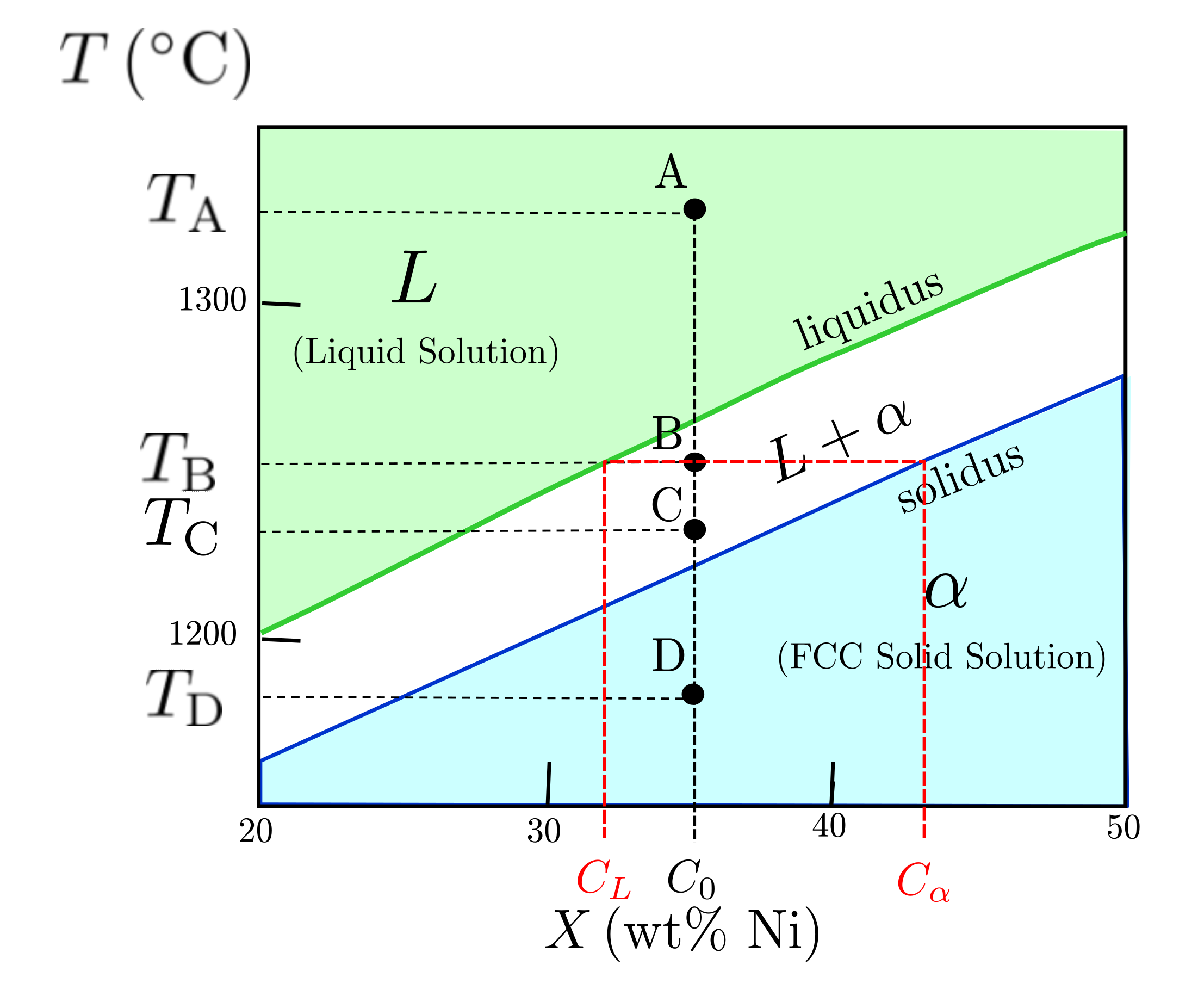
Figure 10.6.3 The application of a tie line to Point B in our phase diagram.
Phase Fractions
What if we want to find the fraction of our mixture that is comprised of each phases? Again, we have two points that are simple because they are single-phase regions, but one that is more complicated.
In general, we denote some phase fraction as $P_i$, where $P$ is the fraction of the mixture that is the phase, and $i$ denotes the phase of interest (e.g. $L$ or $\alpha$). The most common way we see phase fractions reported is as weight fraction $W_i = \frac{m_i}{m_\text{tot}}$, where $m_i$ is the mass of the the phase $i$ and $m_{\text{tot}}$ is the total mass of the system. We'll use that analysis here.
- Point A: We have a single phase, just liquid. So our weight fraction for the liquid phase is simply $W_{L} = 1.0$. Since we have just two possible phases, in this phase diagram, we can also say that $W_{\alpha} = 0$ at this point
- Point D: We have a single phase, just liquid. So our weight fraction for the solid phase is simply $W_{\alpha} = 1.0$ and for the liquid phase it is $W_{L} = 0$.
- Point B: We have two phases. How do we do do this? It turns out (click here for a proof, but we don't go into it in detail), that the equilibrium phase diagram is constructed in a very similar way to a teeter-totter, where we have a lever mounted on a fulcrum and two loads on either side, like shown in Figure 10.6.4.

Figure 10.6.4 Equilibrium for a teeter-totter (top), analogous to equilibrium between masses of phases in a phase diagram.
This equilibrium model us what balance of phase fractions and compositions (analogous to masses and spans on a teeter totter) we need in order to maintain equilibrium. This means that we can equilibrate masses and spans $S$ and $R$ in the same way in the two systems:
Intuitively, at the extrema of $R = 0$ and $S = 0$, this makes sense. If $R = 0$, we're at the liquidus, and so we'd expect nearly all liquid phase. Indeed, if $R = 0$, then $W_{L} = \frac{S}{S} = 1$, the weight fraction for the liquid is 1.
If $S = 0$, we're at the solidus and would expect only solid phase. If $S = 0$, then $W_{L} = \frac{0}{R} = 0$, or $W_{\alpha} = \frac{R}{R} = 1$. This makes sense.
So, let's do the calculation for our example:
$$W_{L} = \frac{S}{R+S} = \frac{C_{\alpha}- C_0}{C_{\alpha}-C_{L}} = \frac{43 \text{wt% Ni} - 35 \text{wt% Ni}}{43 \text{wt% Ni} - 32 \text{wt% Ni}} = 0.73$$
We can also calculate $W_{\alpha}$, but we know that $W_{\alpha} + W_{L} = 1$, because we only have two phases, so
$$W_{\alpha} = 1 - W_{L} = 1-0.73 = 0.27$$
Or, you could confirm the calculation using $W_{\alpha}$ explicitly using Eq. 10.6.1.
Summary
Analyzing isomorphous phase diagrams is confusing at first, but it is very algorithmic in the end. You follow the following formula:
- Determine the location of the point of interest on the phase diagram. Is there one phase present or two?
- If there are two phases, draw a tie line between the liquidus and the solidus. The composition of the tie line's intersection with the liquidus gives you the composition of the liquid phase. The intersection of the tie line with solidus gives you the composition of the solid phase.
- Apply the lever rule to find phase fractions.
This will get a bit more complicated with more complex phase diagrams, but this is essentially the way to analyze phase diagrams. Note - we did not address schematic microstructures yet. (Task 4. in Section 10.3), but I'll check your intuition on that below. Let's practice by completing Exercise 10.6.1 by analyzing Point C in Figure 10.6.2.

Figure 10.6.5 A section of the binary isomorphous Ni-Cu phase diagram.

Figure 10.6.6 Proposed student microstructures.