Tensile Behavior of Materials - Stress and Strain
When a force is applied to any material, it will deform, or change shape. Small deformation (i.e., due to small forces) can be imperceptible to the naked eye or to tactile response - often you don't know the material is deforming. Sometimes, when a small enough force is applied and then removed, the material goes back to its original shape: it has an "elastic" behavior. But, for every material, there is some force that can be applied that will yield a permanent change in shape - "plastic" deformation, or even fracture/failure of the material.
In MSE - and many other fields - it is important to 1. understand what's happening during a deformation process so that we can control it and 2. measure the deformation of a material precisely so that we can communicate about it to others.
Here, we'll first address 2. and return to 1. later. By doing this, we can gain a better understanding of what it looks like when materials deform, and get an idea about how to quantify their mechanical properties so we can better communicate about materials' mechanical responses.
There are many different types of mechanical tests, some of them very specific to certain scenarios. (E.g., special tests for adhesive properties of cells to biomaterial surfaces or for eyewear in women's lacrosse or for amusement park railway ride tracks... you get the idea.) The most widely used basic test of materials, however, is the tensile test, in which a specimen is clamped and stretched, in tension, to the point of failure. In these tests, we measure the applied force and the corresponding displacement to ultimately create a stress-strain curve. Figure 11.3.1 shows a picture of a tensile test machine and Video 11.3.1 shows a short video of a tensile test being carried out.
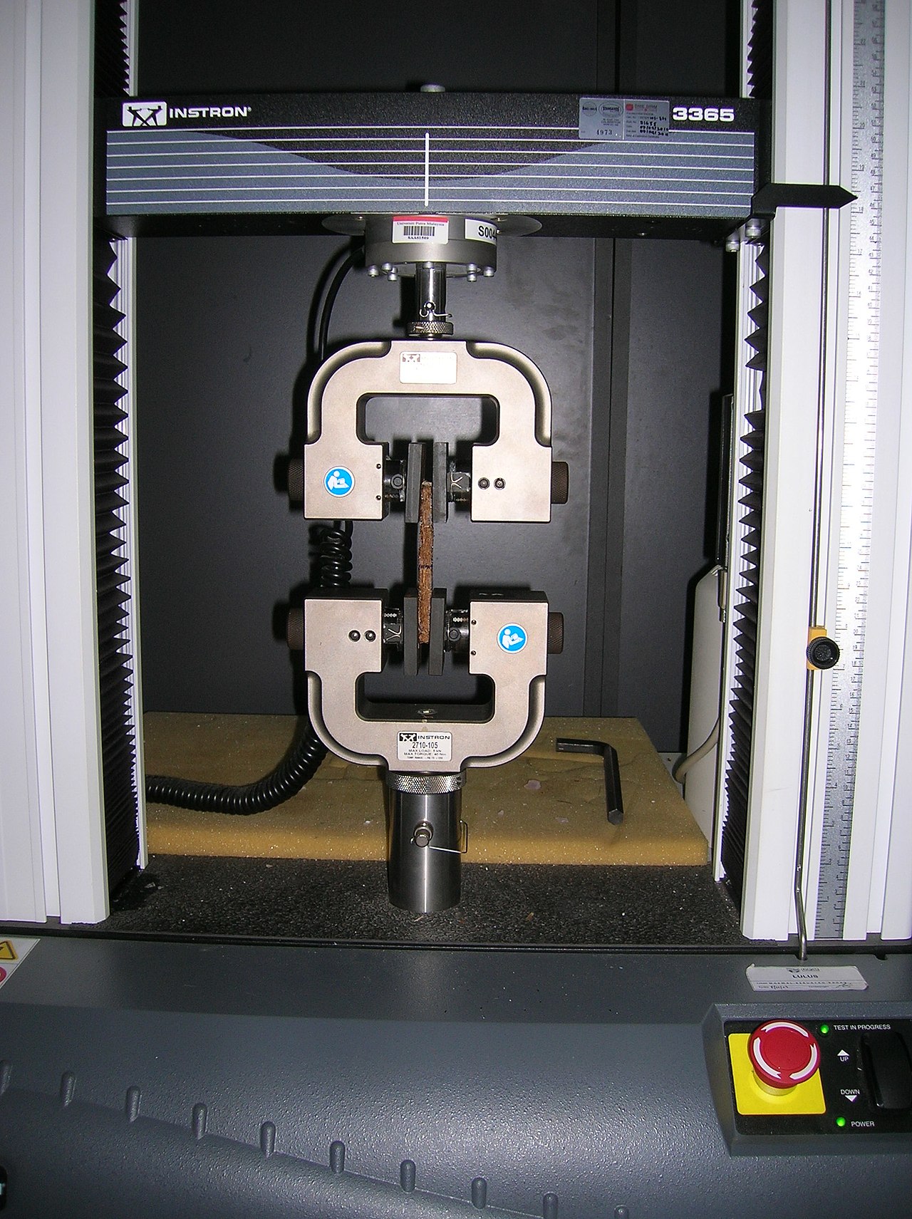
Figure 11.3.1 A tensile test machine
Video 11.3.1
Stress and Strain
The output of a tensile test is a stress $\sigma$ vs strain $\epsilon$ curve. This data is rich in information about all sorts of mechanical properties of the material - stiffness, strength, ductility, toughness, etc - and we'll cover the interpretation of these data in depth in later sections.
The stress-strain curve could obviously depend on the shape and dimensions of the specimen itself. However, as mentioned earlier in the course, we want the property of the material itself. So, we want to ensure that the way we measure the specimen is standardized. The specimen shape, then, is specified to have certain dimensions and shape (often a dog-bone shape with a narrow gauge and broader "shoulders" at the grip, as can be seen in Video 11.3.1). Then, instead of plotting data as force vs displacement (or change in length), data is instead plotted as the stress, which is the force divided by the initial cross-sectional area of the gauge region of the specimen:
$$\sigma=\frac{F_t}{A_0}$$
Where $\sigma$ is the stress, $F_t$ is the applied tensile force and $A_0$ is the initial cross-sectional area. This is illustrated in Figure 11.3.2 Over the course of the measurement, the cross-sectional area of the sample will change, typically thinning, or "necking" as the specimen is stretch. However, it is difficult to measure this change in area during the test (although it can be done), and in most engineering application, the original cross-sectional area $A_0$ is used and the resulting stress is known as the engineering stress. If it were calculated with the instantaneous cross-sectional area (which require constantly measuring it or empirical corrections), it would be the true stress. We'll stick to engineering stress in this course.
We also need a measure of deformation. In a tensile test, we use the strain, which is defined as the change in the length of the sample divided by its original length:
$$\epsilon=\frac{L-L_0}{L_0}=\frac{\Delta L}{L_0}$$
Where $\epsilon$ is strain, $L$ is the current length of the specimen (under load), and $L_0$ is the initial length prior to loading. This is also illustrated in Figure 11.3.2.
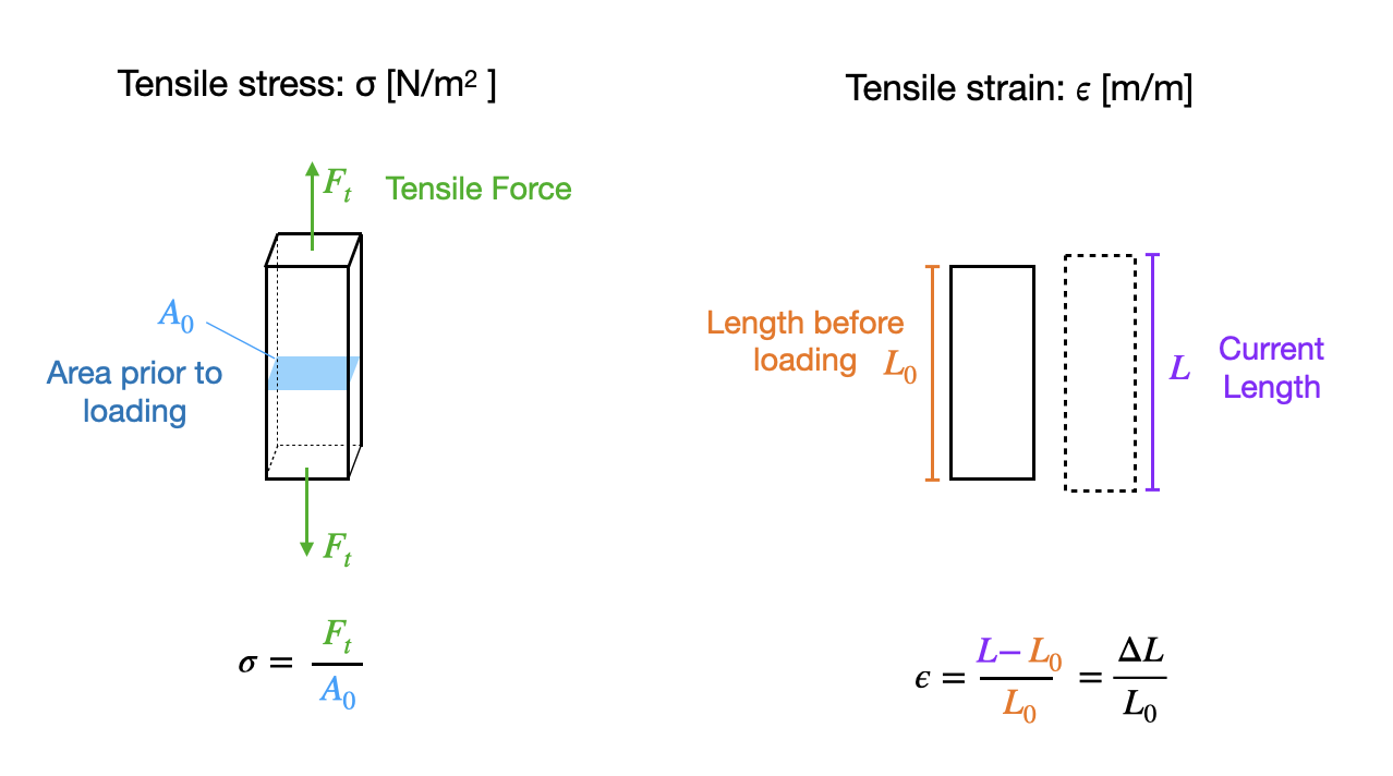
Figure 11.3.2 Tensile stress and tensile strain defined and illustrated.
Strain-Strain curves and other concepts
With the concepts of stress and strain defined above, we can now use the tensile test simulation in NetLogo model 11.3.1 to explore stress-strain curves and some additional concepts. The model is a molecular dynamics model which slowly increases the tensile force applied to the sample over time and plots the stress-strain curve. Use the model to answer Exercise 11.3.1.
Use NetLogo model 11.3.1 to answer the questions below. When you push setup you'll see a small (very small) dogbone specimen of about 50 atoms. This is much, much smaller than actual specimens, of course, be we can still glean some valuable information from this model.
-
Run the model with
auto-increment-force?on. In a sentence or two, describe the shape of the stress-strain curve. Remember, you can speed up or slow down the model as necessary. -
In each of the three regions of the stress-strain curve discussed in the solution to the previous question, what is happening to the bonds of the atoms?
-
- Elastic deformation is deformation of a material (i.e., strain) that disappears when the force is removed (i.e., the material goes back to the shape it was).
- Inelastic deformation (more commonly called plastic deformation ) is deformation/strain that remains permanently after the force is removed.
Based on the model, what is the difference at that atomic level between elastic and plastic deformation?
You may want to try to explore the elastic regime by clicking off
auto-increment forceat some point where you believe no permanent change has taken place. Then, in a region you think permanent deformation has occurred, click offauto-increment forceagain and observe the difference. -
Using the idea of an interatomic potential (e.g., Section 4.6), try to explain the shape of each of the three regions of the stress-strain curve discussed in the solution to the first question and why the material breaks when it does. The graph below helps. It shows both the interatomic potential and the interatomic force for the Lennard-Jones potential (Section 4.5) used in the model plotted against strain instead of interatomic distance. This question is trickier than it might seem, but spend a few minutes giving it your best shot.

Lennard-Jones Interatomic potential and interatomic force plotted vs strain instead of interatomic distance.