The Diffusion Coefficient
Throughout the previous sections, we kept alluding to the "Diffusion Coefficient", $D$, which was essentially the proportionality constant in both Fick's First and Second Laws. Since $D$ tells us how fast diffusion proceeds, and it is associated with a specific material (you can look up $D$ for atoms diffusion in a host material), it's clear it's a pretty important value.
Indeed, everything we've covered up to this point with regards to Fick's Laws is a bit material agnostic. I can solve for flux across a membrane regardless of what material I have using Fick's First Law (and the material's diffusion coefficient). Similarly I can use Fick's Second Law to predict how concentration profiles will evolve for any material.
So, let's consider the coefficient $D$, now, and where it comes from. Remember, $D$ describes the rate at which diffusion occurs, and based on what we know from Diffusion Mechanisms in Crystalline Solids (Section 7.9), this has everything to do with how an atom can hop from one lattice site to another (whether via vacancies or via interstitial sites).
Since the frequency of the hopping determines $D$, it implies that the diffusion coefficient depends on the energetic barrier to jump from its current site to it's new site. We can conceive of this as some sort of energetic barrier separating two energy-equivalent states. For example, an atom jumping from one octahedral site in a BCC crystal to another will have identical surroundings in both positions: the energy of the two positions is therefore identical. The transition from one octahedral site to another, however, will require host atoms get pushed out of the way, so there is an energetic barrier to diffusion based on this "saddle point" in which the lattice is distorted or coordination is low. We call the maximum energy during this transition the activation energy, $Q$.
Fig. Figure 7.10.1 shows a cartoon of this process. Typically, vacancy-mediated diffusion has a higher activation energy because more bonds are broken and lattice distortions can be large (although the lattice distortion isn't depicted much in this particular figure). Interstitial diffusion often has a lower $Q$.

Figure 7.10.1 The activation energy for diffusion in our two diffusion mechanisms: vacancy-mediated diffusion (top) and interstitial diffusion (bottom). In each case, the transitional state, when an atom is away from its equilibrium position, is at a higher energy. We call the maximium energy at this transitional, or "saddle" point the activation energy, $Q$.
Connection Diffusion and Chemical Reaction
Many of you have seen this in chemistry already, where there's a similar concept: the rate constant of a chemical reaction, $k$. A diffusional hop is really no different, as the rate constant in a chemical reaction is described in the same way. So, you may have encountered this expression for the temperature-dependent rate of a reaction:
Where $E_{\mathrm{A}}$ is the activation energy of the reaction, $R$ is the gas constant, and $A$ is a pre-exponential factor that accounts for collision frequency and other factors.
In diffusion, we have a completely analogous situation in which we write the diffusion coefficient as
Where Q is the activation energy of the diffusional jump (Figure 7.10.1) and $D_0$ is a temperature-independent pre-exponential factor that accounts for materials-dependent factors like vibrational modes in a crystal, jump distances between sites entropic contributions, etc. These values are measured and tabulated, but for this introductory course, we won't delve into the details of $D_0$ - we teach fives weeks on this later in the MSE Core Sequence at Northwestern, and it is a bit beyond the scope here. We'll use these $D_0$ values, but we won't derive its source rigorously.
Working with Arrhenius Behavior
Both Eq. 7.10.1 and Eq. 7.10.2 are of the same form, but they're a bit difficult to work with in their exponential form. As such, it is a common practice to transform any Arrhenius behavior into a linear form by eliminating the exponential term:
$$ \begin{align} D &= D_{\text{0}}\,\text{exp}\left(- \frac{Q}{R T}\right)\\ \text{ln} D &= \text{ln} D_{\text{0}}- \frac{Q}{R}\left(\frac{1}{T}\right) \end{align} $$
This may not seem very useful, but it is! This is because now the equation is a linear form. We can plot $\ln{D}$ vs $1/T$ and get a line with slope of $Q/R$ and an offset of $\ln{D}$. So, instead of working with a complex exponential function (left side of Figure 7.10.2) we can instead work with the plot on the right side of Figure 7.10.2, using it to extract relevant values $Q$ for different diffusional systems. This is indeed how we have historically found different values of $D$ for systems of interest! A researcher would measure $D$ experimentally at different temperatures, plot the value on the Arrhenius plot, and derive $Q$. This process has allowed us to extract diffusion coefficients experimentally over the last 70+ years, supplying researchers and engineers with the necessary data to help design processing of ceramics, polymers, metals, and composites.

Figure 7.10.2 A graphical representation of the transformation of the exponential Arhennius equation to a linear form (as in Section 7.10.6).
Figure 7.10.3 shows some examples of some real diffusion data. Notice some interesting features! A drop around $900 ^{\circ}\mathrm{C}$ when C or Fe diffuse in iron, a much higher diffusion coefficient for interstitial diffusion mechanisms, a clear temperature dependence, and clear changes in activation energy for different structures and diffusional behaviors.
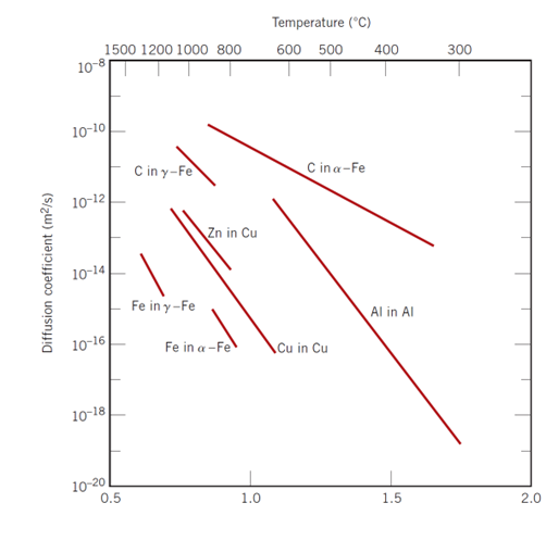
Figure 7.10.3 Diffusion data for a few different systems.